Machine learning using Clojure, libpython-clj2, and Pytorch
Motivation
The Clojure programming language has desirable properties for software engineering such as immutability and strong support for implementing parallel algorithms. Currently Python is popular for machine learning due to Pytorch and other machine learning libraries targeting the Python programming language. However using libpython-clj2 one can invoke Pytorch for machine learning from within Clojure.
This article demonstrates a few basics of machine learning using the \(y=x^2\) parabola function as an example.
Import PyTorch
The PyTorch library is quite comprehensive, is free software, and you can find a lot of documentation on how to use it. The default version of PyTorch on pypi.org comes with CUDA (Nvidia) GPU support. There are also PyTorch wheels provided by AMD which come with ROCm support. Here we are going to use a CPU version of PyTorch which is a much smaller install.
You need to install Python 3.10 or later. For package management we are going to use the uv package manager. The following pyproject.toml file is used to install PyTorch and NumPy.
[project]
name = "mlp"
version = "0.1.0"
description = "Provision Pytorch CPU"
authors = [{ name="Jan Wedekind", email="jan@wedesoft.de" }]
requires-python = ">=3.10.0"
dependencies = [
    "numpy",
    "torch",
]

[tool.uv]
python-preference = "only-system"

[tool.uv.sources]
torch = { index = "pytorch" }
numpy = { index = "pytorch" }

[[tool.uv.index]]
name = "pytorch"
url = "https://download.pytorch.org/whl/cpu"

[build-system]
requires = ["setuptools", "wheel"]
build-backend = "setuptools.build_meta"
Note that we are specifying a custom repository index to get the CPU-only version of PyTorch. Also we are using the system version of Python to prevent uv from trying to install its own version which lacks the _cython module. To freeze the dependencies and create a uv.lock file, you need to run
uv lockYou can install the dependencies using
uv syncIn order to access PyTorch from Clojure you need to run the clj command via uv:
uv run cljNow you should be able to import the Python modules using require-python.
(require '[tablecloth.api :as tc]
         '[scicloj.tableplot.v1.plotly :as plotly]
         '[libpython-clj2.require :refer (require-python)]
         '[libpython-clj2.python :refer (py. py.-) :as py])
(require-python '[builtins :as python]
'[torch :as torch]
'[torch.nn :as nn]
'[torch.utils.data :as data]
'[torch.nn.functional :as F]
'[torch.optim :as optim]):okThe training data
First we are going to set the random seed for reproducibility of this article.
(torch/manual_seed 1)<torch._C.Generator object at 0x7fa0cc1ad090>We are going to sample a small set of points from the interval \([-2, +2]\) and add Gaussian noise to the labels.
(def extent 2.0)(def n 64)(def noise 0.25)(def features (torch/sub (torch/mul (torch/rand [n 1]) (* 2 extent)) extent))(def labels (torch/add (torch/mul features features) (torch/mul noise (torch/randn [n 1]))))(torch/squeeze features 1)tensor([ 1.0305, -0.8828, -0.3877, 0.9387, -1.8829, 1.1994, -0.4115, 1.0175,
0.2780, -0.2449, 0.5547, 0.0987, 0.7305, -0.7794, -0.1458, -0.1801,
0.2899, -0.0080, 1.7483, 0.6224, -0.7448, -1.2079, -0.3352, -0.8627,
-0.6409, 0.0958, 1.1923, 1.0871, -1.9551, 1.2398, 0.5587, 1.8971,
1.3201, -1.8223, -1.9016, -0.9647, 1.7562, -0.3331, 0.8559, -0.9294,
1.9624, -0.8462, 1.4998, 0.0237, -1.0536, 1.0280, -1.0616, 0.5882,
-0.5775, -0.2193, -1.9228, -0.9536, 1.0853, -0.4862, 1.9921, 1.6032,
-0.0936, -1.3350, 1.2179, 0.6207, -1.2928, 1.2991, 1.2142, 1.7738])(torch/squeeze labels 1)tensor([ 1.0556e+00, 5.2343e-01, 1.2828e-03, 6.2985e-01, 3.4926e+00,
1.4368e+00, 5.8765e-01, 1.0379e+00, -9.8686e-02, 1.3654e-02,
5.8658e-02, -1.9808e-01, 4.1831e-01, 4.6745e-01, 1.2016e-01,
-2.1315e-01, -4.2587e-02, 2.5008e-02, 2.8932e+00, 5.7028e-01,
1.9615e-01, 1.3339e+00, 1.5529e-01, 7.0422e-01, 4.7441e-01,
-1.1632e-01, 1.1612e+00, 1.3648e+00, 3.5603e+00, 1.4195e+00,
3.8496e-01, 4.0967e+00, 1.9081e+00, 3.6182e+00, 3.8203e+00,
7.0220e-01, 3.4306e+00, -9.2481e-02, 5.0070e-01, 1.1418e+00,
4.1850e+00, 8.6712e-01, 2.2237e+00, -3.7243e-02, 5.8463e-01,
9.0184e-01, 7.5752e-01, 6.2636e-02, 5.5197e-01, -9.1986e-02,
4.0185e+00, 1.1135e+00, 1.2291e+00, 3.1262e-01, 4.1024e+00,
2.4624e+00, 6.4830e-01, 1.7238e+00, 1.4800e+00, 8.5044e-01,
1.1763e+00, 2.1373e+00, 1.4997e+00, 3.2313e+00])Next we are going to combine features and labels into a PyTorch dataset.
(def dataset (data/TensorDataset features labels))In order to check that the model generalises well, one usually splits up the available data into a training, development and test set.
(def train-size (int (* 0.6 n)))(def dev-size (int (* 0.2 n)))(def test-size (- n train-size dev-size))The random_split function is used to randomly split the dataset.
(def splits (data/random_split dataset [train-size dev-size test-size]))(def train-ds (nth splits 0))(def dev-ds (nth splits 1))(def test-ds (nth splits 2))The datasets are used in the following way:
- training data is used to train the model
- development data is used to check that the model is not overfitting or underfitting
- test data is used to report the performance of the model
Next we are going to use PyTorch DataLoaders to split training and development data into mini-batches. The data loaders are also used to shuffle the data sets. Shuffling can be quite important for stability of the training process.
(def train-data-loader (data/DataLoader train-ds :batch_size 4 :shuffle true))(def dev-data-loader (data/DataLoader dev-ds :batch_size 4 :shuffle true))(def test-data-loader (data/DataLoader test-ds :batch_size test-size :shuffle true))The Model
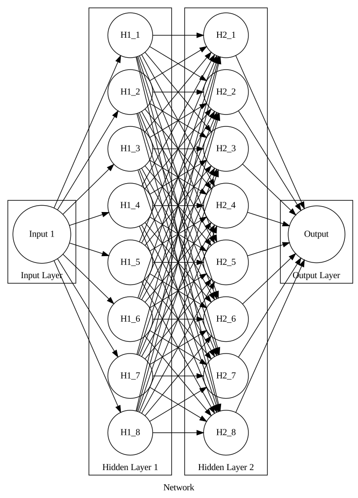
In Python you can implement a small neural network with an input layer, two hidden layers, and an output layer as follows:
class ParabolaNet(nn.Module):
    def __init__(self, n_hidden):
        super().__init__()
        self.fc1 = nn.Linear(1, n_hidden)
        self.fc2 = nn.Linear(n_hidden, n_hidden)
        self.fc3 = nn.Linear(n_hidden, 1)

    def forward(self, x):
        x = self.fc1(x)
        x = F.sigmoid(x)
        x = F.dropout(x, p=self.dropout_rate, training=self.training)
        x = self.fc2(x)
        x = F.sigmoid(x)
        x = F.dropout(x, p=self.dropout_rate, training=self.training)
        x = self.fc3(x)
        return x
Using libpython-clj2 one can create the Python class from within Clojure.
(def ParabolaNet
  (py/create-class
    "ParabolaNet" [nn/Module]
    {"__init__"
     (py/make-instance-fn
       (fn [self n-hidden dropout-rate]
           (py. nn/Module __init__ self)
           (py/set-attrs!
             self
             {"dropout_rate" dropout-rate
              "fc1" (nn/Linear 1 n-hidden)
              "fc2" (nn/Linear n-hidden n-hidden)
              "fc3" (nn/Linear n-hidden 1)})
           nil))
     "forward"
     (py/make-instance-fn
       (fn [self x]
           (let [x (py. self fc1 x)
                 x (F/sigmoid x)
                 x (F/dropout x :p (py.- self dropout_rate) :training (py.- self training))
                 x (py. self fc2 x)
                 x (F/sigmoid x)
                 x (F/dropout x :p (py.- self dropout_rate) :training (py.- self training))
                 x (py. self fc3 x)]
             x)))}))
Each arrow represents a weight stored in the fully connected layers fc1, fc2, and fc3. There are different layer types in PyTorch. A fully connected layer is the most basic one. To be able to model non-linear functions, activation functions are used (here: sigmoid). The model looks like this when using 8 units in each hidden layer.
When evaluating a model, you should disable gradient accumulation. Otherwise gradients will leak into subsequent training steps. In Python this looks like this:
with torch.no_grad():
    ...
In Clojure we can define a macro to disable gradient accumulation:
(defmacro without-gradient
  [& body]
  `(let [no-grad# (torch/no_grad)]
     (try
       (py. no-grad# ~'__enter__)
       ~@body
       (finally
         (py. no-grad# ~'__exit__ nil nil nil)))))
Now one can perform a model prediction as follows:
(def model (ParabolaNet 10 0.0))(without-gradient
(py. model eval)
(model (torch/tensor [0.0])))tensor([-0.0908])The following function plots all data points (training, development, and test set) and the model predictions for different inputs.
(defn plot-model
  [features labels model]
  (without-gradient
    (py. model eval)
    (let [x   (range (- extent) (+ extent 0.01) 0.01)
          y   (map (fn [x] (py. (first (model (torch/tensor [x]))) item)) x)
          ds  (tc/dataset {:x x :y y})
          pts (tc/dataset {:x (map first (py/->jvm (py. features tolist)))
                           :y (map first (py/->jvm (py. labels tolist)))})]
      (-> ds
          (plotly/base {:=title "Model"})
          (plotly/layer-point {:=dataset pts :=x :x :=y :y :=name "data"})
          (plotly/layer-line {:=x :x :=y :y :=name "prediction"})))))
Before training, the model should just be a random function.
(plot-model features labels model)Using the test set, we can report the performance of the model. Note that it is good practice to use a separate test set to report performance, because hyperparameter tuning using the dev set can overfit the model to the dev set.
(defn report-perf
  [model test-data-loader]
  (without-gradient
    (let [[features labels] (first test-data-loader)
          prediction        (model features)
          errors            (torch/sub prediction labels)]
      {:n (builtins/len errors)
       :min (py. (torch/min errors) item)
       :mean (py. (torch/mean errors) item)
       :max (py. (torch/max errors) item)
       :std (py. (torch/std errors) item)})))
(report-perf model test-data-loader){:n 14,
:min -3.883366346359253,
:mean -0.9666337966918945,
:max 0.1055092141032219,
:std 1.0836751461029053}Note that the output is not zero. PyTorch performs random initialisation of the weights for us. Breaking the symmetry like this is important, otherwise all activations and gradients will be the same and the model will not be able to learn.
Training
A training epoch performs the following step for each mini-batch in the training set:
- reset the gradient of the optimizer
- perform model predictions for the input features
- compute the loss which compares the predictions with the labels
- perform backpropagation to get gradients for each model parameter
- perform a gradient descent step using the optimizer
- return the loss value
(defn train-epoch
  [train-data-loader criterion model optimizer]
  (py. model train)
  (for [[features labels] train-data-loader]
       (do
         (py. optimizer zero_grad)
         (let [prediction (model features)
               loss       (criterion prediction labels)]
           (py. loss backward)
           (py. optimizer step)
           (py. loss item)))))
In order to check whether the model is overfitting or underfitting, we need to evaluate the model on the development set. The following method computes the loss values for each mini-batch in the development set.
(defn dev-epoch
  [dev-data-loader criterion model]
  (py. model eval)
  (without-gradient
    (for [[features labels] dev-data-loader]
         (let [prediction (model features)
               loss       (criterion prediction labels)]
           (py. loss item)))))
We define a function to compute the average of a list of numbers.
(defn average [numbers]
  (/ (reduce + numbers) (count numbers)))
Now we can implement a training run. A training run basically consists of many training epochs. Here we are using the stochastic gradient descent method (SGD). Note that usually the Adam optimizer is used, because it is more efficient. As a loss function we simply use the mean squared error (MSE).
(defn training-run
  [train-data-loader dev-data-loader epochs n-hidden lr dropout-rate]
  (let [model     (ParabolaNet n-hidden dropout-rate)
        optimizer (optim/SGD (py. model "parameters") :lr lr)
        criterion (nn/MSELoss)]
    (loop [epoch 1 train-losses [] dev-losses []]
          (let [train-loss (average (train-epoch train-data-loader criterion model optimizer))
                dev-loss   (average (dev-epoch dev-data-loader criterion model))]
            (if (< epoch epochs)
              (recur (inc epoch) (conj train-losses train-loss) (conj dev-losses dev-loss))
              {:model model :train-losses (conj train-losses train-loss) :dev-losses (conj dev-losses dev-loss)})))))
Let’s train a model.
(def learning-rate 0.1)(def num-epochs 20000)(def n-hidden 64)(def result (training-run train-data-loader dev-data-loader num-epochs n-hidden learning-rate 0.0))Hyperparameter tuning
Let’s plot our model.
(plot-model features labels (:model result))As one can see, the model is overfitting the training set. I.e. the model fits the training data closely but does not generalize well. This makes the model sensitive to noise.
Here one can observe overfitting directly. In general however one uses the training and dev loss to detect if the model is overfitting.
First we define a smoothing function which smoothes a sequence of loss values.
(defn smoothing
  [alpha]
  (fn [coll]
      (reductions (fn [prev-avg current] (+ (* alpha prev-avg) (* (- 1 alpha) current))) 0.0 coll)))
Next we define a function to plot the training loss (learning curve) and validation loss over time.
(defn plot-losses
  [{:keys [train-losses dev-losses]} smoothing-fn]
  (-> (tc/dataset {:x (range 1 (count train-losses)) :y (smoothing-fn train-losses)})
      (plotly/base {:=title "Losses"})
      (plotly/layer-line {:=x :x :=y :y :=name "training loss"})
      (plotly/layer-line {:=dataset (tc/dataset {:x (range 1 (count dev-losses)) :y (smoothing-fn dev-losses)})
                          :=x :x :=y :y :=name "dev loss"})))
Let’s plot the losses without smoothing.
(plot-losses result (smoothing 0.0))In practice one uses smoothing to make the trend of the curves more visible.
(plot-losses result (smoothing 0.99))Of particular interest are the loss values at the end of the training process.
(last (:train-losses result))0.034154752967879176(last (:dev-losses result))0.13410548369089761As one can see, the final dev set loss is more than twice the amount of the training loss. This is a sign that the model is overfitting (high variance).
High variance can be resolved using the following techniques:
- use more data
- regularization
- neural network architecture search
We can report the performance using the test set.
(report-perf (:model result) test-data-loader){:n 14,
:min -0.30802178382873535,
:mean 0.11105262488126755,
:max 0.5724084377288818,
:std 0.2797224223613739}Let’s see what underfitting looks like.
(def result2 (training-run train-data-loader dev-data-loader num-epochs 1 learning-rate 0.0))(plot-model features labels (:model result2))Let’s look at the losses.
(plot-losses result2 (smoothing 0.99))(last (:train-losses result2))0.8137271299958229(last (:dev-losses result2))1.8136223355929058As one can see, both the training and dev set loss are high. This is a sign that the model is underfitting (high bias).
High bias can be resolved using the following techniques:
- bigger network
- train longer
- neural network architecture search
We can report the performance using the test set.
(report-perf (:model result2) test-data-loader){:n 14,
:min -2.526854991912842,
:mean 0.6758203506469727,
:max 1.5044240951538086,
:std 1.0056211948394775}Regularization
Instead of tuning the number of hidden units and layers (which can only be done in discrete steps), one can use regularization.
Here we are using dropout regularization which randomly sets some activations to zero during training. After trying out a few values, I found 0.05 to be a good dropout rate for this dataset size and model.
(def result3 (training-run train-data-loader dev-data-loader num-epochs n-hidden learning-rate 0.05))Here is the model output.
(plot-model features labels (:model result3))And the losses are as follows.
(plot-losses result3 (smoothing 0.99))(last (:train-losses result3))0.08883395940065383(last (:dev-losses result3))0.06939788286884625Again we can report the performance using the test set.
(report-perf (:model result3) test-data-loader){:n 14,
:min -0.376054048538208,
:mean -0.01708267442882061,
:max 0.34027233719825745,
:std 0.20343200862407684}Learning Rate
We did not explore different learning rates, but this hyperparameter is usually straightforward to tune:
- The learning rate is too low if the model converges very slowly.
- The learning rate is too high if the loss becomes unstable and the parameters diverge.
Enjoy! :)
source: src/mlp/main.clj